I had a very specific reason for wanting to do this. I was making a prop list, and each item had its own unique ID number, and I wanted to be able to double-check, especially after the list got long, or if any of the ID’s got out of order (maybe they were sorted by page instead?), that there weren’t any duplicate ID’s.
An easy way to avoid update mistakes after a long day of rehearsal.
This prop list happened to be in google sheets, so this tutorial is only in google sheets, but if you can do it in sheets, you can usually do it even easier in Excel.
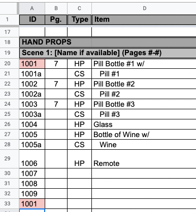 |
This is an example of a sheet I might be working on. And while I was going numerically on the ID’s, I accidentally retyped 1001, rather than 1010. And my formula allowed google sheets to give me a gentle heads up there was a duplicate. |
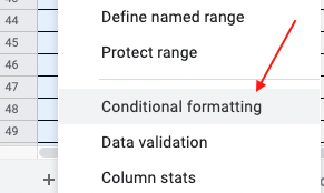 |
Right Click on the highlighted column, and choose (near the bottom) “Conditional Formatting” |
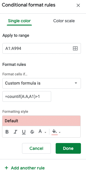 |
Then Add a new rule.
The range should be the whole column (in this case, A1:A994). And I chose to turn it red. |
Note: This works for letters, numbers, or combinations. It is literally comparing the cells, not just comparing the numbers or anything like that.