So this might only ever apply to one specific task, but I’ve done it 2 years in a row now, and I hate having to rediscover things I only do yearly… There also might be a better way to do this, but I don’t know what it is!

So, I have a spreadsheet template that was used last year, and I want to make the same template into next year. [The one I’m working with may have originally been a google template]. It comes with a tiny bit of conditional formatting, which I’ll get to at the end.

So to change the dates, I’m going to simply enter the new date of whatever that first Sunday is.  In this case I typed “8/27/23”:

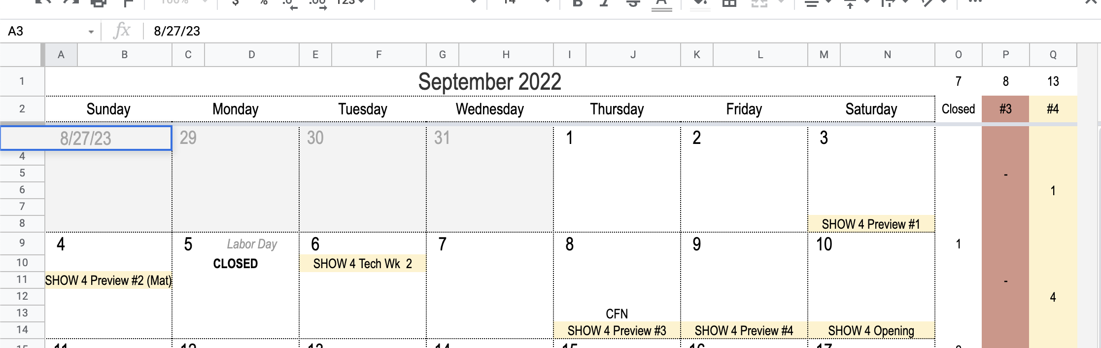
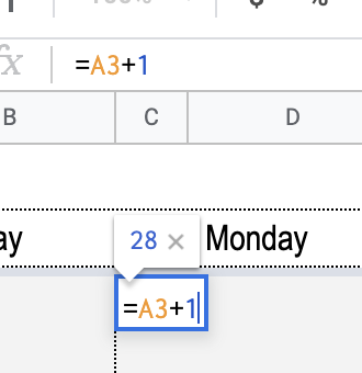
Then on the next cell, I reference the first cell +1 (or “=A3+1”) and it will show us as the 28th.

I then just copy and paste that cell across the row (Sheets will automatically update which cell it’s referencing.

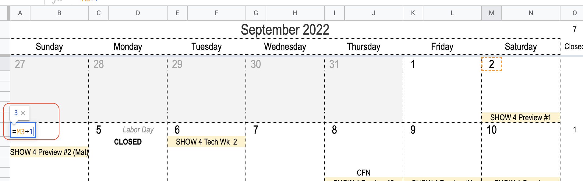
Then on the next week, I start it out by highlighting the last cell from the previous week +1, and then do the formula above for the next 6 days across.

Then I copy and paste the whole row, and put it on the next few rows, until my whole month is complete.

Then I take the days that are actually from a previous month and manually turn them a very light gray.

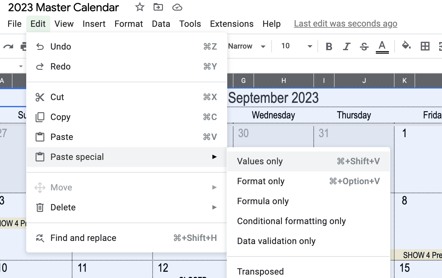
THEN, and it’s important not to forget this step, I copy the entire document, go to EDIT > PASTE SPECIAL > PASTE VALUES. So that if someone highlighted a particular day, they won’t see just a formula.

And then I do that for every month.

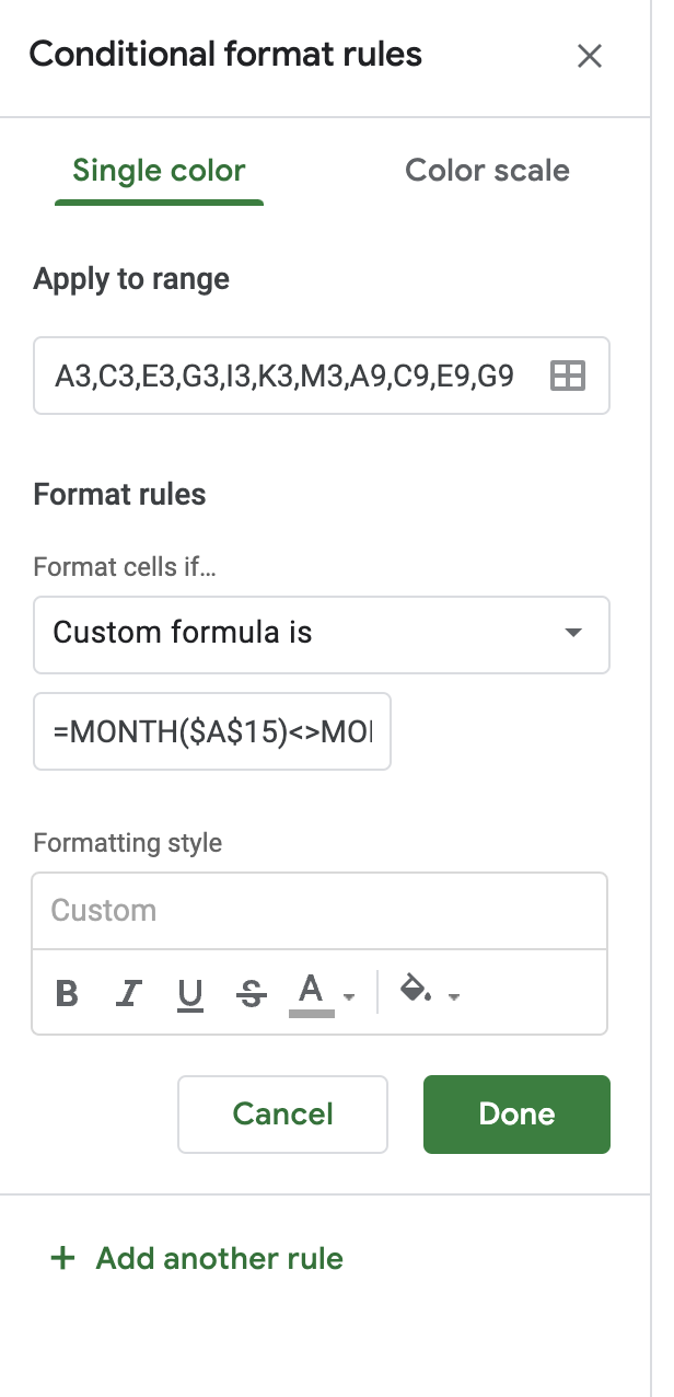
Also worth noting that this template came with a little bit of conditional formatting, to turn THE NUMBER/DATE of days that are on a previous month, a dark gray. The formula selects just the date cells, and in custom formula is “=MONTH($A$15)<>MONTH(A3)”, and the response is to turn the text gray. I just also choose to turn the whole box gray.